Counting the uncountable: a Bayesian Polya urn model for monitoring artisanal fisheries

Here, we establish the notation and fundamental probabilistic structure that support the Bayesian formulation for finite-population inference used in this study. Thus, a finite population of known size N has its elements labelled by i = 1, 2…, N. We further assume these labels as known. It is further characterized by the set I = {Ii; i = 1, 2, …, N} of indicators such that Ii = 1 if unit i is included in a sample or Ii = 0 otherwise. The elements i of this population are the sampling units. In addition to the indicator Ii, each sampling unit is associated with a quantitative characteristic of interest yi (which may be a vector), forming the study population Y = {yi; i = 1, …, N}. Interest generally lies in parameters expressed as known functions T(Y), such as the population total, mean, median, or standard deviation.

However, these FPP can only be known exactly through a census. If, instead, we define a sample 𝐈𝑠⁢𝑢⁢𝑏={𝐼𝑖1,𝐼𝑖2,⋯,𝐼𝑖𝑛} being s = (i1, …, in) a subset of (1, …, N) of a size n = (dimension of s) ≤ N is drawn from I, the population will be subdivided into the sampled subgroup Ys = {yi; i ∈ s} and the non-sampled subgroup 𝐘𝑠𝑐={𝑦𝑖;𝑖∈𝑠𝑐}. That is, 𝐘={𝐘𝑠,𝐘𝑠𝑐}. The indicators I will be known for the entire population once s is available.

Since 𝑇⁡(𝐘)=𝑇⁡(𝐘𝑠,𝐘𝑠𝑐), it becomes clear that this parameter must now be estimated and relies on inferring 𝐘𝑠𝑐. Therefore, using only the known characteristics of the sample D = (s, Ys), inference methods must be applied to obtain information about the characteristics of 𝑌𝑠𝑐.

In frequentist survey sampling (Cochran 1977; Lumley 2010), inferences about T(Y) are based exclusively on the probability distribution of I, which is induced by the specific sampling design used to collect the sample, while Y is considered fixed. This approach is termed “design-based”. In contrast, the Bayesian approach (Gelman et al. 2015) is “model-based” and treats both I and Y as random variables with a joint distribution:

where θ and ϕ are parameters associated with Y and I, respectively. In BFPI, the central object is the posterior predictive distribution 𝑝⁡(𝐘𝑠𝑐|𝐘𝑠,𝐈).

A solution of major practical relevance arises when the sampling design is irrelevant for inference (ignorability) and the units of Y are exchangeable. We will now formalize the conditions for these properties to hold and define the Polya posterior as a non-informative predictive distribution suitable for inference of T(Y) when these properties are valid.

We use π(·) as probability distributions of hyperparameters θ and ϕ, retaining the notation p(·) for Y or I. The complete likelihood is given by eq. 1 while the observed likelihood is

By Bayes’ theorem, the posterior distribution for the parameters is

However, since interest lies in θ, which parameterizes the distribution of Y, we integrate the above distribution with respect to ϕ:

We assume prior independence between θ and ϕ, i.e., π(θ, ϕ) = π(θ) · π(ϕ). We also assume p(I|Y, ϕ) = p(I|Ys, ϕ), meaning that there is independence between sampling units inclusion probabilities and the quantities of interest associated to, at least, the unobserved fraction of them 𝐘𝑠𝑐. This property is known as the ignorability assumption, which renders the sampling design irrelevant for inferring 𝐘𝑠𝑐 conditional on Ys.

To verify this, we rewrite the last expression, incorporating the assumptions of independence between θ and ϕ and the ignorability of the sampling design:

where the last integral reduces to a normalization constant p(I), and thus I is removed as a conditioning variable in the posterior distribution of θ.

Finally, under an ignorable sampling design, the marginal distribution of Y is

If the elements of Y are independent when conditioned to θ, they are said exchangeable. Thus, under exchangeability of Y, we can write

Substituting into the previous expression and noting that p(Ys|θ)π(θ) = π(θ|Ys)p(Ys), we obtain

However, since

it follows that this integral defines the predictive distribution of 𝐘𝑠𝑐 conditioned on the observed sample values Ys.

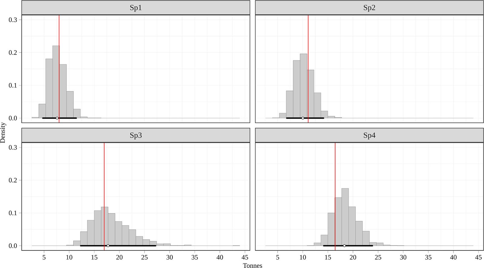
To simulate a sample from this predictive distribution, we proceed in two steps: first, simulate values of θ from the posterior distribution π(θ|Ys), and then simulate values for 𝐘𝑠𝑐 according to the model 𝑝⁡(𝐘𝑠𝑐|𝜃). The T(Y) values associated with these simulations will determine the posterior distribution for this FPP.

An intuitive understanding of exchangeability is useful to assess whether this assumption is reasonable in practical situations. Let Y = {y1, y2, …, yN} with prior probability p(Y). Suppose it is discovered that the unit indices (labels) were misassigned and are actually a permutation I′ of the correct indices I; that is, we are actually referring to Y′ = {y3, y8, …, y2}. If p(Y) = p(Y′) for any Y′ with permuted indices relative to I, then the population Y is said exchangeable.

In the next section, we present a generic and useful method to obtain a predictive distribution, even in cases with insufficient information to formulate a detailed model for Y. Only the assumptions of approximate exchangeability in Y and ignorability about the sampling plan are required.

After observing Ys, we want to obtain the posterior predictive distribution 𝑝⁡(𝐘𝑠𝑐|𝐘𝑠). This conditional probability implies dependence between the sampled and unsampled units and is implicit in the assumption of exchangeability for 𝐘. Ghosh and Meeden (1997) show that this distribution can be easily obtained using a Polya urn model and denote 𝑝⁡(𝐘𝑠𝑐|𝐘𝑠) simply the Polya posterior.

We refer to this distribution simply as

where k are the number of categories, the sample size n is defined by 𝑛=∑𝑘𝑗=1𝑛𝑘, nj are the number of units in Ys that fall in category j, and 𝐘𝑠𝑐 has N − n elements. In fact, when dealing with continuous variables, we use the most extreme case in which each observed Yi defines a distinct category. In this case, k = n and (n1,…, nk) = (1,…, 1) = 1n. For more details see Appendix A.

The Polya urn model is a powerful non-informative Bayesian approach when very little prior information about the population is available. It is non-parametric in the sense that no specific model 𝑝⁡(𝐘) has to be specified once ignorability and exchangeability are acceptable assumptions. If an equal inclusion probability for all units can be ensured, these conditions hold, and the Polya posterior is always valid. However, in general, this condition is sufficient but not necessary. When at least some partial prior information about auxiliary variables is available, the Polya posterior can still yield very satisfactory results without equal inclusion probability, particularly in situations for which standard frequentist procedure are difficult to apply (Lazar et al. 2008).

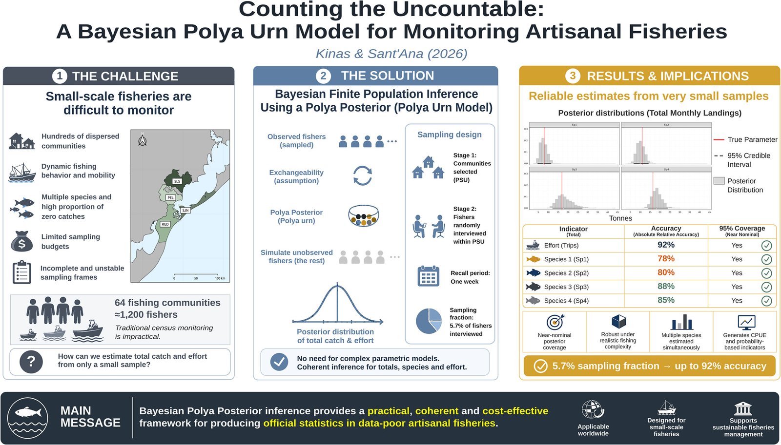
Within the scope of the PLE fisheries, which will be described in more detail in the next section, there were two pre-conditions that would invalidate overall approximate exchangeability. First, the distinct characteristics of the four municipalities. Second, variations in expected landings throughout the 4 weeks where changes in weather conditions, among others, can affect the outcomes. The inclusion of municipality and week as auxiliary variables made it possible to conceptualize approximate exchangeability as reasonable within each of these 16 resulting strata. Here, without loss of generality, we are modelling only the four weekly strata within one municipality, to estimate monthly total landings.

Even after guaranteeing at the outset the same inclusion probability of all fishers over a month period (Section 2.4 for details), the sampling plan split these fishers between weeks, so that any selected fisher would report landings only for one specific (randomly selected) week. This was thought useful for two reasons: first, to obtain better quality data, as it is easier for fishers to remember the activity for 1 week rather than over the whole month; and second, to be less invasive to individual monthly production. Hence, for each sampled fisher, the three missing weeks are not exchangeable with the sampled week.

Across fishers within weeks (as strata), we have overall equal inclusion probabilities for the first week. When working with the sample for the second week, fishers that were previously sampled will have zero inclusion probability. In each subsequent week within a month, the number of fishers with zero-inclusion probability grows. However, we consider it still reasonable to assume approximate exchangeability within a week and build the Polya posterior accordingly. Any frequentist method relaying on expansions based on inclusion probabilities would face difficulties.

We used the polyapost package (Meeden et al. 2024) in R 4.4.2 (R Core Team 2025) to perform the Polya urn simulations. Replicating this procedure M = 1500 times, a simulated Polya distribution will emerge. Finally, for any FPP defined as a known function T(Y) to each of these simulations of 𝐘𝑠𝑐, the Polya posterior distribution for T is obtained. Following advise by Gelman et al. (2021) we included “mad.sd” (rescaled median absolute deviation; formula “1.48*Median(abs(x − median(x))”; implemented in R as function “mad(x)”) as a computational robust estimate to be preferred over “sd”. To measure relative precision we further defined “mad.cv” as the ratio “mad.sd” divided by “median”.

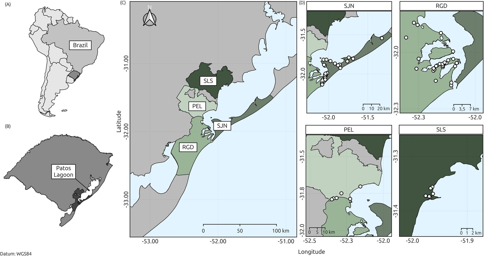
The characteristics that shaped the synthetic population to be used throughout were motivated by the actual artisanal fishery in four municipalities involving the PLE as shown in Fig. 1. The Patos Lagoon is 265 km long with an average width of 40 km. The estuary comprises about 10% of the Patos Lagoon’s total area of 10 227 km2 (Möller et al. 1996).

The 64 communities shown as white circles on the map, are the home of about 1200 fisher and their families. Communities are of different sizes; from the smallest with about 10 fisher to the largest exceeding 100. For sampling purposes, large comnunities were previosly split into sub-groups of at most 55 fisher before sampling. Average distances among communities vary among these municipalities; smallest average 1.3 km, followed by 9.7 km, 10.8 km, and largest 21.9 m. The maximum distance between two communities within the municipality at the right border of the ELP is 97.1 km.

Each municipalities became a stratum, and, as such, it suffices to concentrate here on a synthetic population that features one typical municipality, only. A complete description of the region, the sampling strategy as it was adapted to each stratum, and further details on the monitoring program and results over a 1 year period is currently in preparation.

We consider a population of N = 350 fishers labeled from 1 to N and distributed in 12 communities of varying sizes, from 10 to 50. For a given fisher i ∈ (1, …, N) and week j ∈ (1, 2, 3, 4) within a month, data consist in the weekly total fishing effort fij (e.g., number of fishing operations) and the catch of four fish species ci,j = (ci,j, 1, …, ci,j, 4) in kilograms. For simplicity and without lack of generality, we assume that these four species are exaustive in describing the catch.

The finite population is therefore a dataframe with 350 rows and 22 columns: two columns to label fishers and communities followed by five weekly data columns (fi,j, ci,j) for weeks j ∈ (1, 2, 3, 4).

The FPP of interest are the total monthly effort, and this quantity can be estimated by

and the total monthly catch per species s = 1, 2, 3, 4. That is, given a species s, and adding over all weeks and fisher, the total per species Sps is

Twelve groups of fishers (representing communities) of sizes 10, 40, 10, 20, 50, 30, 20, 30, 30, 10, 50, and 50 were fixed to complete a total population of N = 350. Effort f, here defined as the number of fishing trips within a week, was generated for each fisher from Poisson distributions with averages 4, 0.5, 1.5, and 2.5 for each of the 4 weeks. The overall averages of catch-per-unit effort were fixed within groups for species “Sp1” to “Sp4”, as sampled values in the ranges [35, 45], [3, 7], [85, 115], and [12, 18], respectively. The total weekly catch for each individual fisher was simulated by sampling f times from a Gamma(α/2, 1/2) and adding these f numbers; where α represents the catch-per-unit-effort per species and group. 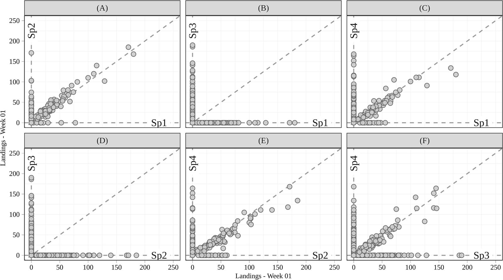Finally, to emulate realistic conditions, we added two other features into the catch simulations: (a) probability of occurrence that vary between species (causing lots of zeros in the data, a very common and annoying feature in practice) and (b) correlations between species (induced by manipulating conditional probabilities of occurrence of some species given others). To achieve both goals, we multiplied each term of the matrix of the just simulated catches, by species occurrence-indicators as defined next. We define x1, x2, x3, and x4 as random quantities simulated from Bernoulli Ber(p) distributions: x1 ∼ Ber(p1 = 0, 30), x2|x1 = 1 ∼ Bern(p21 = 0.90), and x2|x1 = 0 ∼ Bern(p20 = 0.15). In sequence, we defined x3 = (1 − x1)(1 − x2) to indicate that “Sp3” occurs whenever neither “Sp1” nor “Sp2” occur. Finally, x4|x3 = 1 ∼ Bern(p41 = 0.50) and x4|x3 = 0 ∼ Bern(p40 = 0.80). Some graphical displays and statistical summaries that characterize this synthetic population are given in Section 3.1 below.

With the synthetic population at hand, we devised a sampling plan from which FPP could be estimated using a Polya posterior distribution. This sampling plan required a realistic field-work dynamic for which exchangeability and ignorability are valid. The next section describes a slightly simplified version of the sampling plan that is being used in the ELP field work.

The real world logistics required the coverage of large distances among communities, accessibility challenges dependent on weather conditions, and the number of field personnel to do the work.

Since data were collected through interviews, we considered that the report aggregated effort and landings with respect to the week prior to the week of the interview would result in acceptable accuracy due to the short time lag. Furthermore, since weather conditions can change strongly within days, affecting uniformly all fishers in the population, this stratification by week, was expected to improve the required conditions for exchangeability.

Based on all these considerations, in addition to a previous pilot field study described in Kinas and Wieczynski (2020), a probabilitic two-stage sampling was proposed. The first stage in selecting randomly k communities per week with probability proportional to the number possible of permutations of m fishers within the community, and the second stage by sampling m fishers from each selected community. With this procedure the same inclusion probability is achieved for all fishers, irrespective of the community size. Hence, each week a total of k × m fishers were asked to report effort and landings for the previous week.

After 4 weeks, a total sample of size n = 4km fishers composes the data available for inference. Since each sampled fisher reported only 1/4 of her (his) monthly landing, the sampling fraction is in fact n/(4N).

To avoid resampling the same community within a month and to give all fishers the same selection probability, irrespective of their community size, we sample at once all 4k communities without replacement and with probability proportional to the number of combinations of m fishers that could be formed within that community. Finally, to avoid that the larger communities, which are expected to be selected first, tend to fall into weeks one or two, we randomized the order of the eight selected communities before splitting them into four weekly groups of size k. From each selected community, m fishers were selected at random without replacement.

To evaluate the robustness of the Polya posterior estimates when equal sampling inclusion probabilities is invalid, we tested two alternative sampling plans, denoted “A1” and “A2”, with increasing deviation from this core assumption. Sampling plan “A1” selected communities (first stage) with equal probabilities, irrespective of its size but retained random sampling of fishers within communities. As a result, sampling plan “A1” gives higher inclusion probabilities to fishers from smaller communities. Sampling plan “A2” added to “A1” higher inclusion probabilities to fishers with better performance within communities. These inclusion probabilities were defined with a logistic model logit(pi) = β0 + β1xi, where xi is the standardized monthly landing for fisher i and pi is predefined inclusion probability; we used β0 = −2.51 and β1 = 0.19.

The term “calibrated Bayes” was coined by Little (2006) to describe a strategy to combine the Bayesian strength for inference under a given statistical model, with the tools to assess its frequentistic performance. Little’s idea was to combine both paradigms in order to explore the strength of each.

Given our goal of providing sample-based monthly official statistics of aggregated fish catch and total effort, it was important to evaluate the performance of the Bayesian Polya posterior distributions. There are general quality standards, recommended by FAO for design-based statistical sampling monitoring data (Stamatopoulos 2002), which we adapted as tools into a Bayesian calibration mindset.

Using the synthetic population to provide the true FPP, and 300 replications of the sampling plan laid out in Section 2.4, the performance inference could be measured. Hence, our metrics for assessment were defined as follows:

From each replicated posterior Polya distribution j = 1, …, K (where K = 300) and some FPP of interest T, we defined as potential estimates the posterior mean (tj), the posterior median (gj), the 95% percentile credibility interval (CrIj), and the 95% highest posterior density interval (HPDj). The performance of the posterior mean and median as point estimates of T were evaluated by its Absolute Relative Accuracy (ARA), defined as

for the posterior mean with ̅𝑡 denoting the mean of all M replicated posterior means. Similarly ARA(g) and ̅𝑔 refer to the posterior medians. These numbers are expressed as percentages, with maximum accuracy at 100%, while dropping as the estimates worsen. Stamatopoulos (2002) recommends accuracies in the range [90%, 95%] as acceptable for basic fishery statistics.

We further wanted to relate the nominal posterior probability interval to its de facto coverage and precision. Precision being here quantified as the average width of the intervals, while coverage as the relative frequency of all intervals containing T. Ideally, the observed relative frequency should be as close as possible to the nominal value. Stamatopoulos (2002) defines sample precision in terms of the coefficient of variation CV of an estimate, recommending CV < 15% for basic fishery statistics.

We start with some general features of the synthetic population, meaning the characteristics that describe the production and effort for all N = 350 fishers. These fishers are aggregated into 12 communities (clusters) with varying sizes, from 10 to 50. We induced some intra-community correlation that caused average landings and variances within clusters to vary among communities (Table 1).

Overall variations in landings among fish species (i.e., some species dominate landing biomass) and variations among weeks (reflecting, among others, varying weather condition) were further induced and can be checked from the general summaries depicted in Table 2.

To build the synthetic population, we included a typical data structure encountered when dealing with these type of fishery production data. One such feature is the high quantity of zeroes for some species, while others are simultaneously abundant. This feature emerges with changes in fishing ground from one community to another or by the use of distinctive gear types for different target species. Since none of these informations are being collected, they cannot be used to define strata. Finally, another challenge posed to inference is the fact that the vector of all species has to be estimated jointly. In Fig. 2, the overall two-way relations among landings for all four species are displayed for week 1 only (similar features are valid for the remaining weeks; not shown). The fair amount of data points on the vertical and horizontal axes indicate zero-catches for the specific species. For instance, in panel (A), for many registered positive landings for “Sp2” there are no landings for “Sp1”, shown by points on the y axis and similarly for the x axis; furthermore 209 of all 350 data points are on the origin where there are zero-catches for both. The number of points at the origin (joint-zeroes) is 54, 117, 30, 111, and 35 for panels (B)–(F), respectively. Another interesting feature is captured by panels (B) and (D) showing that landings of species “Sp1” and “Sp2” never occur together with “Sp3”. The overall proportion of zero-catches by species is 78% for “Sp1”, 72% for “Sp2”, 54% for “Sp3”, and 52% for “Sp4”.

Given the virtual population, we devised the sampling plan laid out in Section 2.4. Each week, k = 2 communities were randomly selected and m = 10 fishers were randomly selected without replacement within these two communities. Hence, by the end of a month, a total n = 80 fishers from eight communities will have been interviewed. Since each fisher will have reported landings and effort for only one of the 4 weeks, the overall sampling fraction turns out to be 1/4 of n/N, which is 5.7%.

In Fig. 3, the Bayesian posterior estimates for the monthly landings of all four species are displayed together with the true population parameters (red lines), while in Table 3, some numerical marginal posterior summaries along with the true FPP are listed. For this particular sample, all true FPPs fall within the posterior 95% CrI. Posterior median and mean differ slightly reflecting some asymmetry towards heavier upper tails in the marginal posterior distributions; a very common feature for fisheries data (Hilborn and Walters 1992). It shows that some parameters are better estimated than others, by comparison. Furthermore, depending on the targeted species, sample size could be modulated based on these estimates. The last line in Table 3 gives the true “FPP” for comparison.

Before finishing this section, we want to explore some special features that can be easily answered within the Bayesian paradigm and which, in contrast, would be quite challenging in the context of the conventional sampled-based approach. We illustrate with two less usual, but certainly useful, questions to be addressed once the sample has been collected.

The first is an estimate of the Capture per Unit Effort (CPUE), an important concept in fisheries sciences that can be interpreted simply as a measure of fishing efficiency. But under quite general conditions, it is often used as a proxy to population abundance. Hence, it is certainly of interest to evaluate CPUE monthly and display its dynamics over time. Here, we use CPUE of species “Sp2” to illustrate. Based on the Polya posterior of 1500 total monthly effort (“Eff”) and landing of species “Sp2”, we just need to divide the latter by the former to get the required Polya posterior estimate. This posterior distribution is displayed as the left panel in Fig. 4. As in previous cases, the red vertical line is the true CPUE obtained from census data. The 95% CrI spans from 4.6 ton/day to 10.1 ton/day, with median equal to 7.2 ton/day while the “true” value is 8.1 ton/day.

The second question describes the interest in the probability that, in the surveyed month, a given threshold was overrun. For instance, if it were known that the port installation processing capacity is limited to 62 tonnes within a month, it might be of interest to estimate the probability p that this threshold was surpassed by effective landings. To obtain an estimate we simply count the number of times the Polya-simulated estimate for Sp1 + Sp2 + Sp3 + Sp4 exceeds 62 tonnes. Hence, we have M = 1500 responses of which xY are “Yes” and M − xY are “No”. Assuming a Binomial distribution Bin(M, p) for xY and defining a Beta(1, 1) non-informative conjugate prior for p, we obtain a posterior Beta distribution Beta(xY + 1, M − xY + 1) (Gelman et al. 2015). These results are shown in the right panel of Fig. 3 in which the continuous line is the exact posterior Beta distribution. The histogram of a simulated sample from this Beta distribution is also displayed. Based on the sampled fishers, we therefore estimated p at 0.112 (median) with 95% CrI ranging from 0.097 to 0.129. In words, there is an almost 90% chance that the threshold was not reached. In fact, the true total was 52.5 tonnes; below the threshold as we expected to be highly probable.

Calibration was implemented by multiple replications of the sampling plan described in Section 2.4. Each week two communities were selected and 10 fishers within each, comprising 20 fishers per week or 80 per month. For each sample, the Polya posterior was obtained with 1000 replications. The complete procedure was then repeated 300 times. From these 300 replicated inferences, the metrics defined in Section 2.5 were calculated. The results are displayed in Table 4

In Table 4, we see that the simulations of the Polya urn model produced posterior estimates with accuracies ranging from 77% to 92% with a sampling fraction of only 0.057. These results are encouraging, considering that landing data are challenging due to typically containing many zeros alongside occasionally very high values within any single species, together with complex non-conventional correlations among species as was displayed in Fig. 1. Furthermore, and at least for this particular virtual population, the choice between the posterior median and the posterior mean to serve as estimates had negligible effect on the accuracies.

Columns 5 and 7 of Table 4, showed that posterior intervals had 3–5 percentage points lower coverages than the nominal value of 95%. The highest (posterior) density intervals (HDI) exhibited consistently narrower average width in comparison to the credible intervals (CrI) as expected by definition. However, this came at the cost of slightly inferior coverages for three (“Eff”, “Sp1”, “Sp3”) of the five FPP tested.

The effect of sampling plans “A1” and “A2” on the performance of the Polya posterior are summarized in Tables 5 and 6, respectively. There, we present ratios between the average performance measures given the alternative sampling plan divided by its counterpart for the reference sampling plan. Ratios that are larger than 1 indicate higher values for the alternative sampling plan, while ratios lower than 1 indicate the opposite. In Table 5, it showed that unequal sampling inclusion of fishers caused by ignoring the sizes of the communities had mixed effects, as the ratios vary around unity without any clear pattern towards one direction. Thus, suggesting some level of robustness to this sampling plan. The reported average increase of 5% (i.e., Avg ratios of 1.05) for the length of posterior 95% intervals indicates increased posterior uncertainties under “A1” driven mostly by species “Sp1” for which the average length increased about 17%.

In contrast, the negative effect of sampling plan “A2” is clearcut, as summarized in Table 6. The averages of the ratios (last line) show reductions of 4% and 5% in ARA for the posterior median and mean, respectively. The length of posterior intervals increased by 17% although, somewhat surprisingly, the coverages remained about the same; particularly for HDI.